The Bulletproofs protocol allows you to produce these zero-knowledge proofs based only on the discrete logarithm assumption, no trusted setups. This essentially means no pairing (like KZG/Groth16) but a scheme more involved than just using hash functions (like STARKs). This protocol has been used for rangeproofs in Monero, as a polynomial commitment scheme in proof systems like Kimchi (the one at the core of the Mina protocol), and in Zcash's Halo 2. So it's quite versatile as well as well-deployed in the real world.
The easiest way to introduce the Bulletproofs protocol, I believe, is to explain that it's just a protocol to compute an inner product in a verifiable way:
$$\langle \vec{a}, \vec{b} \rangle = c$$If you don't know what an inner product is, imagine the following example:
$$\langle \begin{pmatrix}a_1 \\ a_2 \\ a_3 \\ a_4\end{pmatrix}, \begin{pmatrix}b_1 \\ b_2 \\ b_3 \\ b_4\end{pmatrix}\rangle = a_1 b_1 + a_2 b_2 + a_3 b_3 + a_4 b_4$$Using Bulletproofs makes it faster to verify a proof that $\langle \vec{a}, \vec{b} \rangle = c$, rather than computing the inner product yourself. But more than that, Bulletproofs even lets you hide one or both of the inputs, or the output, to obtain interesting ZK protocols.
Furthermore, if computing an inner product doesn't sound that sexy by itself, you can imagine that it is used to do actual useful things like proving that a value lies within a given range (a range proof), or even that a circuit was executed correctly (when used within a general-purpose zero-knowledge proof system). But this is out of scope for this explanation :)
Alright, enough intro, let's get started. Bulletproofs and its variants always "compress" the proof by hiding everything in commitments, such that you have one single point that represents each input/output:
- A = $\langle \vec{a}, \vec{G} \rangle$
- B = $\langle \vec{b}, \vec{H} \rangle$
- C = $\langle \vec{a}, \vec{b} \rangle Q $
where you can see each point $A, B, C$ as a non-hiding Pedersen commitment with independent bases $\vec{G}, \vec{H}, Q$ (so the above calculations are multi-scalar multiplications). To drive the point home, let me repeat: single points instead of long vectors make proofs shorter!
Because we like examples, let me just give you the commitment of $\vec{a}$:
$$\langle \begin{pmatrix}a_1 \\ a_2 \\ a_3 \\ a_4\end{pmatrix}, \begin{pmatrix}G_1 \\ G_2 \\ G_3 \\ G_4\end{pmatrix}\rangle = a_1 G_1 + a_2 G_2 + a_3 G_3 + a_4 G_4$$Different protocols (like the halo one I talk about in the first post) since bootleproof (the paper that came before bulletproofs) aggregates commitments differently. In the explanation above I didn't aggregate anything, but you can imagine that you could make things even smaller by having a single commitment $P = A + B + C$ to the inputs/output.
At this point, a prover can just reveal both inputs $\vec{a}, \vec{b}$ and the verifier can check that they are valid openings of $A, B$, and that $c = \langle \vec{a}, \vec{b} \rangle$ is a valid opening of $C$. If we had aggregated all commitments into a single commitment $P$ then you would check that aggregated opening.
But as I said earlier, this is not very efficient (you have to perform the inner product as the verifier) and it also is not very compact (you have to send the long vectors $\vec{a}$ and $\vec{b}$).
I know it's also not zero-knowledge, but we will just explain Bulletproofs/IPA without hiding, and for the hiding part we'll just ignore it as we usually do when handwaving explanations of ZKP schemes.
That being said, the prover will eventually send the two input vectors in the clear, but before doing that they will reduce them. More precisely, the prover and the verifier will do this dance to reduce, together, the problem statement $\langle \vec{a}, \vec{b} \rangle = c$ to a much smaller $\langle \vec{a'}, \vec{b'} \rangle = c'$ where the vectors $\vec{a'}$ and $\vec{b'}$ both have a single entry.
If the original vectors were of size $2^n$ then Bulletproofs will perform $n$ reductions in order to get that final statement (as each reduction halves the size of the vectors), and then will send these "reduced" input vectors $a',b'$. At this point the verifier will produce $c' = \langle a', b' \rangle$ and check that they are valid openings of the reduced commitments $A', B'$ and $C'$.
If you've followed until now, you should now be expecting that we need to answer the following two questions next:
-
how does the reduction from $A, B, C$ to $A', B', C'$ work?
-
how is it verifiable?
To reduce stuff, we do almost the same basic operation that we like to do in every "folding" protocol: we split our vector in half and produce a random linear combination of the two halves. Except that here we'll have to also use the inverse $x^{-1}$.
Note The need for the inverse of $x$ is because we're dealing with a much harder algebraic structure, Pedersen commitments, which as pointed in this post are basically random linear combinations of what you're committing to (hidden in the exponent). This makes it hard to perform any linear combinations of its entries without producing wrong results due to the randomness. Fortunately, the use of $x^{-1}$ will nicely allow us to "cancel out" annoying terms as will become apparent very soon.
Here's how we'll fold our inputs:
- $\vec{a'} = x^{-1} \begin{pmatrix}a_1 \\ a_2\end{pmatrix} + x \begin{pmatrix}a_3 \\ a_4\end{pmatrix}$
- $\vec{b'} = x \begin{pmatrix}b_1 \\ b_2\end{pmatrix} + x^{-1} \begin{pmatrix}b_3 \\ b_4\end{pmatrix}$
Then you get two new vectors $\vec{a'}, \vec{b'}$ of half the size. This means nothing much so far, so let's look at what their inner product looks like:
$$ \begin{align} \langle \vec{a'}, \vec{b'} \rangle =& \langle \begin{pmatrix}x^{-1} a_1 + x a_3 \\ x^{-1} a_2 + x a_4 \end{pmatrix}, \begin{pmatrix}x b_1 + x^{-1} b_3 \\ x b_2 + x^{-1} b_4 \end{pmatrix} \rangle \\\ =& (a_1b_1 + a_2b_2 + a_3b_3 + a_4b_4) + x^{-2} (a_1b_3 + a_2b_4) + x^2 (a_3b_1 + a_4b_2) \\\ =& \langle \vec{a}, \vec{b} \rangle + x^{-2} (L) + x^2 (R) \end{align} $$for some cross terms $L$ and $R$ that are independent of the challenge $x$ chosen (so when we will Fiat-Shamir this protocol, the prover will need to produce $L$ and $R$ before sampling $x$).
Wow, did you notice? The new inner product depends on the old one. This means that as a verifier, you can produce the reduced inner product result in a verifiable way by computing
$$\langle \vec{a'}, \vec{b'} \rangle = \langle \vec{a}, \vec{b} \rangle + \text{stuff}$$If what you have is a commitment $C = \langle \vec{a}, \vec{b} \rangle Q$, then you can produce a reduced commitment $C' = C + \text{stuff}$ where "stuff" is essentially provided by the prover, and is not going to mess with $C$ because of the challenge that's shifting/randomizing that garbage (it'll look like $x^{-2} [L] + x^2 [R]$ where $[L]$ and $[R]$ are commitments to $L$ and $R$).
So we tackled the question of how do we reduce, in a verifiable way, the result of the inner product. But what about the inputs? Today's your lucky day because you can use the same trick for the commitment of $a$ and $b$! So essentially, you get $[\vec{a'}] = \text{reduce}([\vec{a}], x, \text{stuff})$ (and similarly for $\vec{b}$).
We can go over it in a quick example, but it'll pretty much look the same as we did above with the addition of having to reduce the generators $\vec{G}$ and $\vec{H}$ as well.
Let's start with reducing the generators, let's just show how to do it with $\vec{G}$:
$$\vec{G'} = x \begin{pmatrix}G_1 \\ G_2\end{pmatrix} + x^{-1} \begin{pmatrix}G_3 \\ G_4\end{pmatrix}$$Now let's look at what a Pedersen commitment of our reduced first input $\vec{a'}$ looks like:
$$ \begin{align} \vec{A'} =& \langle \vec{a'}, \vec{G'} \rangle \\\ =& (x^{-1} a_1 + x a_3)(x G_1 + x^{-1} G_3) + (x^{-1} a_2 + x a_4)(x G_2 + x^{-1}G_4) \\\ =& A + x^{-2} (a_1 G_3 + a_2 G_4) + x^2 (a_3 G_1 + a_4 G_2) \\\ =& A + x^{-2} L_a + x^{2} R_a \end{align} $$In other words, $\langle \vec{a'}, \vec{G'} \rangle = \langle \vec{a}, \vec{G} \rangle + \text{stuff}$ (and similarly for the second input).
Note that in the Bulletproofs protocol, we're dealing with a single commitment $P = A + B + C$ and so we'll reduce that statement to $P' = P + \text{stuff}$ where stuff contains the aggregated $L$ and $R$ for all of the separate commitments.
So just a recap, this is what you're essentially doing with this first round of the protocol:
-
we start from $P = \langle \vec{a}, \vec{G} \rangle + \langle \vec{b}, \vec{H} \rangle + \langle \vec{a}, \vec{b} \rangle Q$
-
the prover produces the points $L$ and $R$
-
the verifier samples a challenge $x$
-
they both produce $P' = P + x^{-2} L + x^2 R$
At this point the prover can choose to release $\vec{a'}$ and $\vec{b'}$ and the verifier can check that this is a valid opening of $P'$ by comparing it with the expected opening $\langle \vec{a'}, \vec{G'} \rangle + \langle \vec{b'}, \vec{H'} \rangle + \langle \vec{a'}, \vec{b'} \rangle Q$.
Bulletproofs doesn't stop there, instead it notices that the reduced statement looks like another statement you could give to Bulletproofs. So in the full protocol, the prover and the verifier reduce the original statement many times, until they get reduced inputs of size $1$. In practice, of course, you can stop earlier.
Warning Notice that we computed $\langle \vec{a'}, \vec{b'} \rangle Q$ which is important because you want to make sure that the inner product result is indeed $\langle \vec{a'}, \vec{b'} \rangle$ and not some arbitrary value. Checking this in the reduced form tells you with high probability that this is true as well in the original statement $P$.
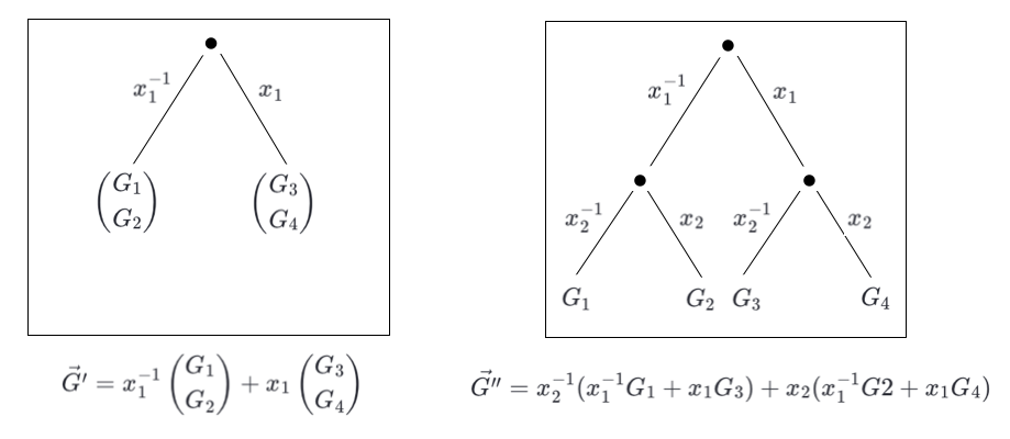
One final detail, in real-world implementation, the reductions are not checked one by one by the verifier, instead all the reduction checks are aggregated into a single check. This means that the verifier knows, based on the challenges seen during the many rounds/reductions of the protocol, how to directly compute the final reduced generators, inputs, and cross-terms.
You can quickly see that by taking a simple example: two rounds of generators folding. The diagram below shows you that the eventual product of challenges that will find themselves in front of every reduced element (in this case the generators comprising the vector $\vec{G}$) can be seen as the path taken by a binary tree of challenges:
In the next part, we'll see how things connect in a sagemath playground!