Optimizing Barrett Reduction: Tighter Bounds Eliminate Redundant Subtractions

Barrett reduction is a widely used algorithm for reducing a value modulo $m$. Our analysis, conducted during the Rust p256 crate audit, shows that the error bound for Barrett reduction can be tighter than traditionally assumed. For most moduli used in cryptography (e.g., NIST curves), the quotient approximation error is at most 1 (not 2). This improvement eliminates the need for a second subtraction in practice. By adopting this optimization, RustCrypto p256 achieves a 14% performance improvement in scalar multiplication.

What Is Barrett Reduction?

Barrett reduction is a method for efficiently computing the remainder of a division operation (i.e., modulus operation), $x \mod m$, without performing an actual division.

We want to compute $r = x \mod m$, which can be expressed as $x = q \cdot m + r$, where $q$ is the quotient and $r$ is the remainder. In practice (e.g., cryptographic field arithmetic), the modulus $m$ can be a large integer represented using $k$ limbs. Each limb is a 32-bit or 64-bit value (depending on the machine word), making the radix $b = 2^{32}$ or $2^{64}$. In practice, the value $x$ is a $2k$-limb integer because it results from the multiplication of two $k$-limb integers.

One way to compute $r$ is to first calculate $q$ as:

Once $q$ is determined, $r$ can be computed as $r = x - q \cdot m$. Barrett reduction provides a more efficient way to approximate $q$, avoiding the need for direct division, which is computationally expensive.

First, let's rewrite the formula above as:

So far, our computation is exact. However, instead of computing $q$ exactly, we'll approximate it by computing:

This allows us to precompute $\mu = \lfloor \frac{b^{2k}}{m} \rfloor$ and rewrite the above as:

Note: Both $\lfloor \frac{\cdot}{b^{k-1}} \rfloor$ and $\lfloor \frac{\cdot}{b^{k+1}} \rfloor$ are fast to compute using right shifts.

Since the two approximations can be smaller than their exact computations, we have $\tilde{q} \leq q$. Traditional analysis has shown that $\tilde{q} \in [q - 2, q]$ (we will elaborate on this in the analysis section). This means the approximate quotient $\tilde{q}$ is at most 2 less than the true quotient $q$.

Computing $r$ in $x \approx \tilde{q} \cdot m + r$

If we had computed $q$ exactly, we would simply compute:

Since $r \in [0, m)$, only the bit length of $m$ is involved in that subtraction. Thus, we can compute it faster by involving only the least significant $b^k$ bits:

(where modulo $b^k$ can be computed efficiently)

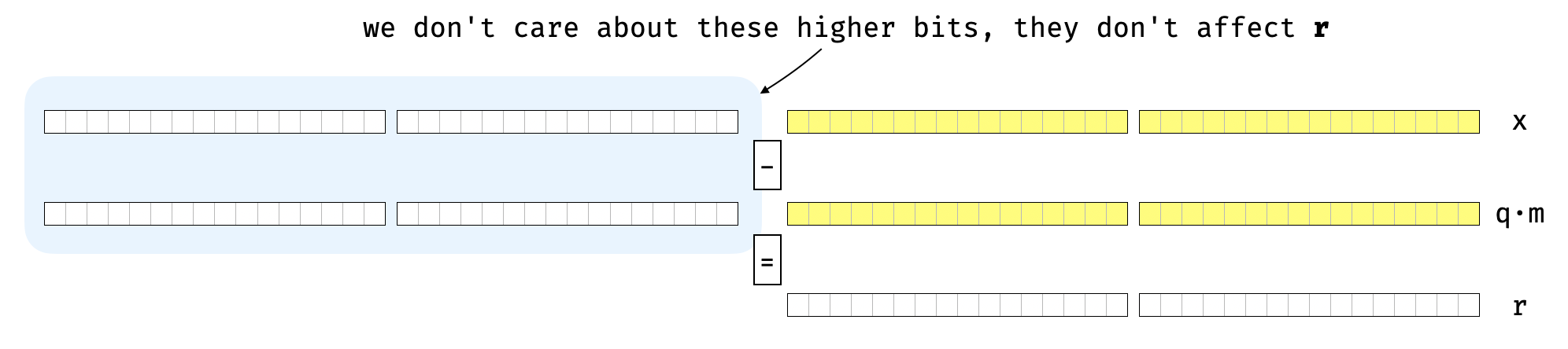
However, remember that we have computed an approximation $\tilde{q}$ of $q$, where $\tilde{q} \in [q-2, q]$.

We know that either:

1. $r = x - \tilde{q} \cdot m$
2. $r = x - (\tilde{q} + 1) \cdot m$
3. $r = x - (\tilde{q} + 2) \cdot m$

To compute $r$, we first calculate case 1. If the result is not smaller than $m$, we subtract $m$ once or twice to bring it into the correct range.

This means that we might not have $\tilde{r} = x - \tilde{q} \cdot m < b^k$ immediately. Instead, the value could be $m$ or $2m$ times larger.

Since $m < b^k$, we know $2 \cdot m < 2 \cdot b^k$. This allows us to upper bound our approximation:

Then, we can calculate $\tilde{r}$ more efficiently:

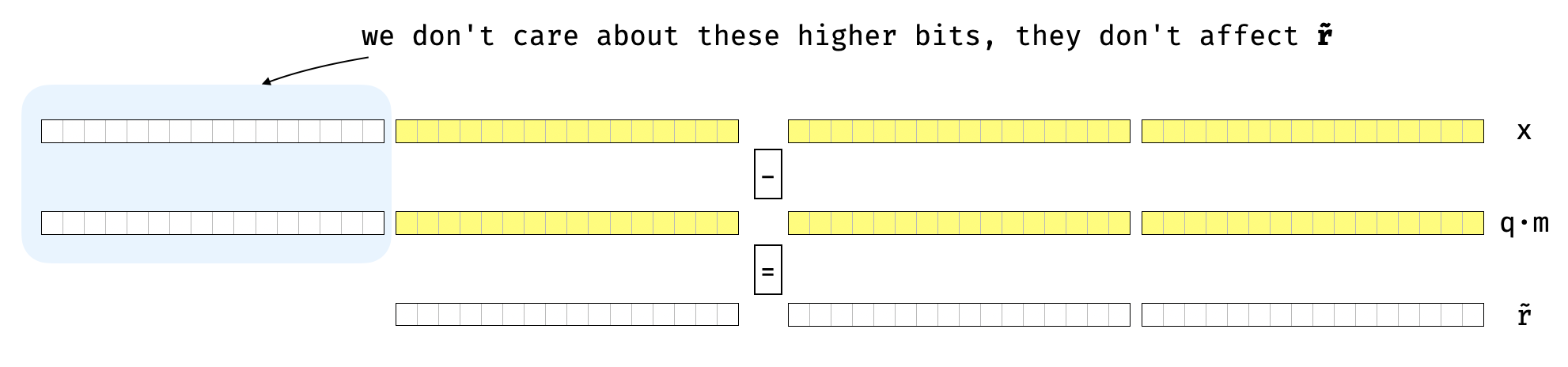
Again, the $\bmod{b^{k+1}}$ operation is very efficient on binary machines.

We finally arrive at the algorithm as described in Handbook of Applied Cryptography, Chapter 14. The steps outlined above closely follow the process detailed in the book.

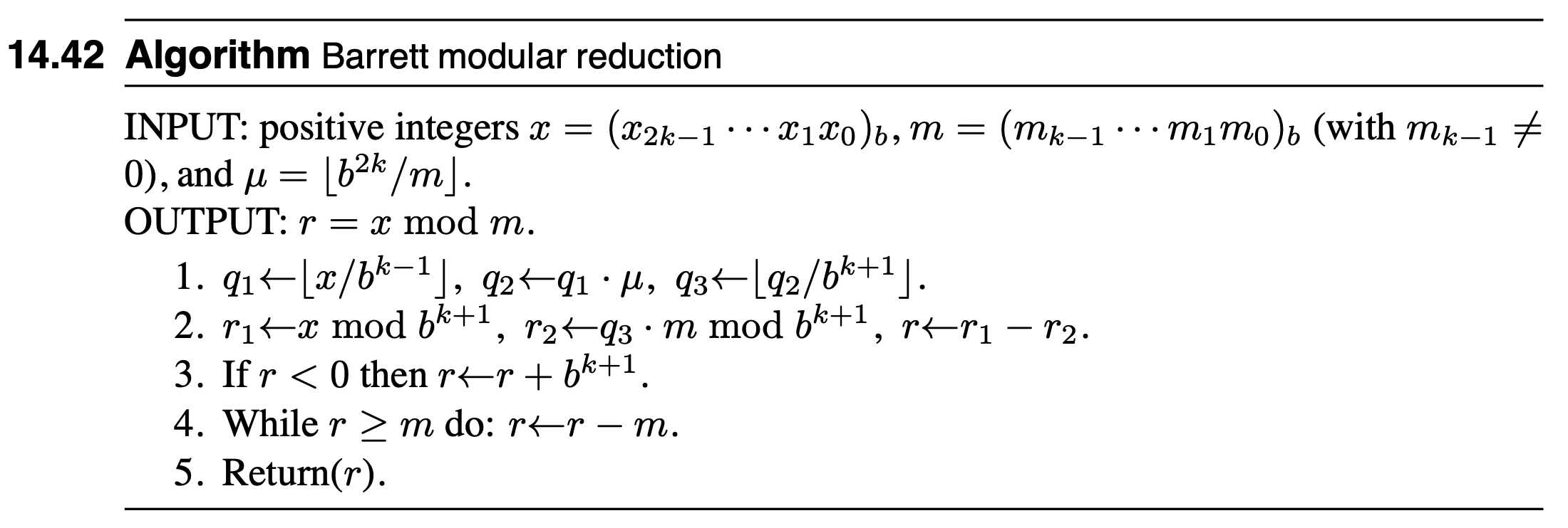
Source: Handbook of Applied Cryptography, Chapter 14

A Tighter Bound Analysis

The bound of $\tilde{q}$ directly determines how many times $r$ needs to be subtracted by $m$ to fall within the correct range. Traditionally, the bound is known to be $\tilde{q} \in [q-2, q]$. In this section, we will show that for almost all moduli in practice, the tighter bound holds: $\tilde{q} \in [q-1, q]$.

Remember that

Since $\tilde{q}$ is derived from a truncated approximation of $\frac{x}{m}$, it naturally satisfies $\tilde{q} \le q$.

Let's denote $\alpha = x \mod {b^{k-1}}$, where $\alpha \lt b^{k-1}$. Denote $\beta = b^{2k} \mod m$, where $\beta \lt m$. Then we can remove the floor operation:

Then we can simplify $\tilde{q}$:

We use ${\color{red}{z}}$ to denote the red part (note that $z \ge 0$). Then we have $\tilde{q} = \lfloor \frac{x}{m} - {\color{red}{z}} \rfloor$. By the floor function inequality $\lfloor x \rfloor + \lfloor y \rfloor + 1 \ge \lfloor x + y \rfloor$, we have:

That is saying $\tilde{q} + \lfloor z \rfloor + 1 \ge q$.

The bound of $z$ is the key to analyzing the bound of $\tilde{q}$. If we can prove that $0 \le z \lt 2$, then we will have $\lfloor z \rfloor \le 1$ and finally $\tilde{q} + 2 \ge \tilde{q} + \lfloor z \rfloor + 1 \ge q$. Let's analyze the bound of $z$.

Prove that $\tilde{q} \in [q-2, q]$

We have:

We know that $b^{k-1} \lt m$ (because $m$ is $k$-limb) and $\beta \lt m$. Then we have:

And thus:

That's exactly what we want. Therefore, we conclude that $\tilde{q} + 2 \ge \tilde{q} + \lfloor z \rfloor + 1 \ge q$.

Tighter Bound in Practice: $\tilde{q} \in [q-1, q]$

We have proved that $\tilde{q} \in [q-2, q]$ under all circumstances. However, this is a loose bound. Here, we claim that for almost all moduli $m$ in practice, we have a tighter bound: $z \lt 1$, and thus $\tilde{q} + 1 \ge \tilde{q} + \lfloor z \rfloor + 1 \ge q$.

Let's examine which moduli $m$ satisfy this tighter bound. Recall that $z \lt \frac{b^{k-1} + \beta}{m}$, so $z \lt 1$ holds if the following is true:

Which means:

Further:

That's saying if $\beta$ is no greater than $m-b^{k-1}$, then $z \lt 1$ and thus $\tilde{q} \in [q-1, q]$. We can formalize this as the Tighter Bound Criterion:

It's worth noting that $\beta = b^{2k} \mod{m}$ falls within $[0, m)$. In practice, where $b$ is either $2^{32}$ or $2^{64}$, and $m$ approaches $b^k$, the value $m - b^{k-1}$ is very close to $m$.

The behavior of $\beta = b^{2k} \bmod{m}$ resembles a uniform random distribution over $[0, m)$ for any random modulus $m$. This makes it highly probable that $\beta \le m - b^{k-1}$. Consequently, most moduli $m$ will satisfy $z \lt 1$, leading to $\tilde{q} + 1 \ge q$.

To quantify this probability, let's assume the common case where $\frac{b^k}{2} \lt m \lt b^k$ and $\beta$ follows a uniform distribution. Under these conditions:

To put this in perspective:

• When $b = 2^{32}$, the probability of achieving the tighter bound exceeds $1 - \frac{1}{2^{31}}$.
• When $b = 2^{64}$, the probability of achieving the tighter bound exceeds $1 - \frac{1}{2^{63}}$.

That is, for nearly all moduli in practice, the tighter bound $\tilde{q} \in [{q-1}, q]$ holds.

Here is an intuitive explanation: $\mu$ (i.e., $\lfloor \frac{b^{2k}}{m} \rfloor$) is the quotient of $m$ divide $b^{2k}$, and $\beta$ is the remainder. If $\beta$ is very small, then $\mu$ will be very close to the actual quotient and thus the calculation of $\tilde{q}$ will have less approximation errors. Our analysis shows that as long as $\beta$ is no greater than $m - b^{k-1}$, the calculated $\tilde{q}$ is at most $1$ less than $q$. As that is a very loose requirement for $\beta$ (or $m$), most of the moduli have a tighter bound.

Practical Optimization For Barrett Reduction Implementation

The tighter bound enables faster Barrett reduction implementation. According to traditional analysis, we may need to subtract $r$ by $m$ twice to get the final result. For a given modulus $m$, if the tighter bound holds, then we can subtract $r$ by $m$ at most once. This means we can save one subtraction.

This is very useful for constant time implementation where it always substract the max times. For example, in RustCrypto P-256 scalar field implementation, it always subtracts twice.

pub(super) const fn barrett_reduce(lo: U256, hi: U256) -> U256 {
    [...]

    let r1 = [a0, a1, a2, a3, a4];
    let r2 = q3_times_n_keep_five(&q3);
    let r = sub_inner_five(r1, r2);

    // Result is in range (0, 3*n - 1),
    // and 90% of the time, no subtraction will be needed.
    let r = subtract_n_if_necessary(r);
    let r = subtract_n_if_necessary(r);
    U256::new([r[0], r[1], r[2], r[3]])
}

As P-256 scalar field satisfies $\beta \le m - b^{k-1}$, the tighter bound $\tilde{q} \in [{q-1}, q]$ holds. This implies the calculated $\tilde{q}$ is at most $1$ less than the actual quotient $q$. This means r can be subtracted at most once to get the final result. The second subtract_n_if_necessary call in the code above is unnecessary and can be safely removed.

Benchmarks show that simply removing the second subtraction improves multiplication and inversion performance by 14%.

scalar operations/mul
    time:   [38.900 ns 38.957 ns 39.026 ns]
    change: [-14.379% -14.052% -13.734%] (p = 0.00 < 0.05)
    Performance has improved.
scalar operations/invert
    time:   [20.716 µs 20.758 µs 20.823 µs]
    change: [-14.817% -14.331% -13.969%] (p = 0.00 < 0.05)
    Performance has improved.

As analyzed in the previous section, the tighter bound holds for almost all moduli. Thus, this optimization applies to most of the Barrett reductions with fixed moduli (e.g., ECC, ZKP).

Here is the Python script to test if a modulus $m$ has the tighter bound:

# Tighter Bound Criterion for the Barret reduction
def tighter_bound_criterion(m):
    def inner_test(m, b):
        # k chosen such that b^{k-1} < m < b^k
        k = 1
        while b**k < m:
            k += 1
        print("k = ", k)
        beta = b**(2*k) % m

        # calculate criterion
        return beta <= m - b**(k-1)

    # test both b=2^32 and b=2^64
    return inner_test(m, 2**32) and inner_test(m, 2**64)

# P-256 scalar field
assert(tighter_bound_criterion(0xffffffff00000000ffffffffffffffffbce6faada7179e84f3b9cac2fc632551) == True)

# P-256 base field
assert(tighter_bound_criterion(0xffffffff00000001000000000000000000000000ffffffffffffffffffffffff) == True)

Conclusion

Our analysis demonstrates that the error bound for the quotient approximation $\tilde{q}$ can be tightened from $[q-2, q]$ to $[q-1, q]$ for almost all moduli used in practice. This tighter bound eliminates the need for a second subtraction in most cases, enabling faster and more efficient implementations.

We showed how this optimization applies to real-world cryptographic libraries, such as RustCrypto's P-256 scalar field implementation, where removing the unnecessary subtraction improved performance significantly. These findings are broadly applicable to other cryptographic systems and zero-knowledge proof frameworks that rely on fixed moduli.